

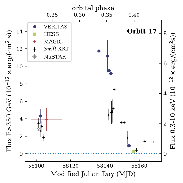
Orbit of the pulsar with location of the shock-nose (upper), and X-ray light curve (lower). See Figure 6 (below) for more details.
Reference: Y.M. Tokayer et al. (The NuSTAR, MDM, and VERITAS Collaborations), Astrophysical Journal 923, 17 (2021)
Full text version
ArXiv: ArXiV: 2110.01075
Contacts: Raul Prado
In this paper, we follow up on the puzzling gamma-ray binary HESS J0632+057 with combined observations by VERITAS, the X-ray observatories NuSTAR and Swift and the optical observatory MDM. The observations are interpreted in two different approaches. First, a two-population leptonic model is used to describe the orbit-folded X-ray light curve and secondly, a pulsar-wind model is fitted to the observed SED over 5 epochs. The results show a good agreement between model and observations and provide a number of quantitative insights about this fascinating system.
FITS files: N/A
Figures from paper (click to get full size image):

Figure 1: Swift light curve folded to an orbital period of 317.3 days, with t0 = MJD 54857.0, the date of the fi
rst Swift-XRT observation. Each data point represents one Swift-XRT observation. 1σ errors are shown. Vertical lines indicate the phases of the NuSTAR (red), VERITAS (blue), and MDM (green) observations. swiftNu2, Ve2, and MDM observations were all during the same 2019-2020 orbit, while the Nu1 and Ve1 observations were of the same orbit in late 2017.

Figure 2: SED derived from NuSTAR observations. The solid lines show the result of the single power law fi
t and the gray band its 1σ confi
dence interval. Values of the integrated flux and spectral index can be found in Table 1.

Figure 3: SED derived from VERITAS observations. Upper plot shows the 2017 data (Ve1a and Ve1b) and bottom plot shows 2019/20 data (Ve2a, Ve2b and Ve2c). Values of the fluxes can be found in Table 2.

Figure 4: Selected regions of the summed optical spectra listed in Table 3. In each panel, the counts spectra are normalized to 1 and shifted by 1 for display purposes. Orbital phase φ
is calculated using the ephemeris of Fig. 1. Interstellar Na I λλ5889; 5895 absorption was used as a wavelength reference. Double-peaked He I λ5876 emission has a peak separation of ≈250 km s-1.

Figure 5: Equivalent widths of Hα
and Hβ
emission lines from Table 3. Orbital phase φ
is calculated using the ephemeris of Fig. 1.
Figure 6: Top: Assumed orbit of the pulsar (black) and location of the shock nose (blue). The relative magnetic fi
eld strength at the nose as a function of phase is indicated in red by radial distance from the pulsar. The cyan dotted line shows the observer LoS, and the cross section of the inclined disk is indicated by the red dashed line. Green curves illustrate the cross sections of the IBS at a few phases for reference. Bottom: A binned X-ray light curve (data points) and light-curve model (black). Each model component (red: orbit+disk, blue: beaming) is also displayed.

Figure 7: PIMMS prediction of Swift-XRT count rates for each NuSTAR observation, overlaid onto the folded light curve. Vertical red lines correspond to the phases of the NuSTAR observations, and horizontal blue lines indicate the predicted Swift-XRT count rates. Intersections for corresponding observations are marked with a green dot. Top: NH = 0.30x1022 cm-2 for all PIMMS estimates Bottom: Adjusted PIMMS estimate for Sw1a using NH = 1.0x1022 cm-2.

Figure 8: Illustration of the orbit of the compact object projected onto the orbital plane for the solutions from Casares et al. (2012a) (solid red line) and Moritani et al. (2018) (dashed blue line) and from Sec. 4 (dash-dotted green line). See Archer et al. (2020) for the complete list of system parameters for the former two. The locations of the compact object during the combined NuSTAR and VERITAS observations of the 2017 and 2019/20 campaign are indicated as black markers. The companion star is assumed to be in a
fixed position and the estimated size of the circumstellar disk (Moritani et al. 2015; Zamanov et al. 2016) is indicated by a dotted black line.

Figure 9: SED data-model comparison assuming the best solution of the model
fitting for the orbital solutions from Casares et al. (2012a) (solid red line), Moritani et al. (2018) (blue dashed line) and from Sec. 4 (green dotted line).