The response of imaging atmospheric Cherenkov telescopes to incident γ-ray-initiated showers in the atmosphere changes as the telescopes age due to exposure to light and weather. These aging processes affect the reconstructed energies of the events and γ-ray fluxes. This work discusses the implementation of signal calibration methods for the Very Energetic Radiation Imaging Telescope Array System (VERITAS) to account for changes in the optical throughput and detector performance over time. The total throughput of a Cherenkov telescope is the product of camera-dependent factors, such as the photomultiplier tube gains and their quantum efficiencies, and the mirror reflectivity and Winston cone response to incoming radiation. This document summarizes different methods to determine how the camera gains and mirror reflectivity have evolved over time and how we can calibrate this changing throughput in reconstruction pipelines for imaging atmospheric Cherenkov telescopes. The implementation is validated against seven years of observations with the VERITAS telescopes of the Crab Nebula, which is a reference object in very-high-energy astronomy. Regular optical throughput monitoring and the corresponding signal calibrations are found to be critical for the reconstruction of extensive air shower images. The proposed implementation is applied as a correction to the signals of the photomultiplier tubes in the telescope simulation to produce fine-tuned instrument response functions. This method is shown to be effective for calibrating the acquired γ-ray data and for recovering the correct energy of the events and photon fluxes. At the same time, it keeps the computational effort of generating Monte Carlo simulations for instrument response functions affordably low.
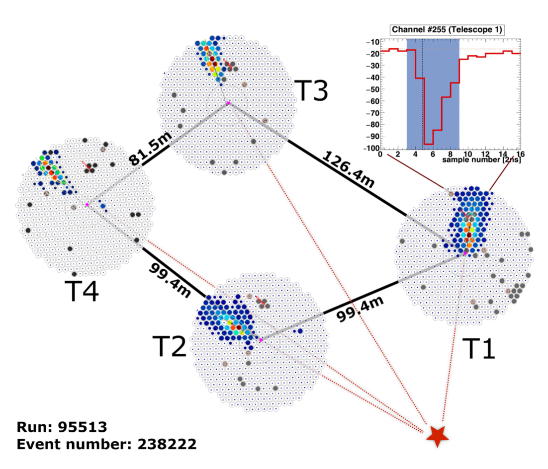
Figure 1: Extensive air shower reconstructed by the VERITAS telescopes. The shower images for each camera have been integrated over time and cleaned using a two-level filter. Dead and disabled channels are shown in dark gray and brown respectively. The signal registered by each PMT is color-coded, with red colors representing higher signal than blue tones. An approximate geometrical reconstruction of the shower core location is illustrated with red dashed lines and a red star. The upper
right plot shows the trace of one of PMT (#255) of T1 for reference. There, the signal registered for each sample of 2 ns is plotted in red and the integration window (six samples) is shown in shadowed blue.
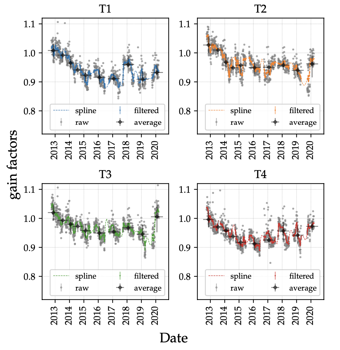
Figure 2: Time-dependent changes of photo-statistic gains normalized to the nominal absolute gains used in the baseline MC model for the current detector model. This detector model was constructed in 2012, and reproduces the characteristics of VERITAS after the PMT camera upgrade. Black points show the average gain factors for each instrument epoch. Gray points show the individual unfiltered gain factor values per telescope and daily flasher run. Blue, orange, green and red points show the result of a median filter of the individual gain factors. Curves of the same colors represent a spline interpolation of the filtered values. Even though spline interpolation can locally diverge when there is no data available, we note that this occurs only during Summer breaks, where
no data is taken in VERITAS, therefore it is not a concern for this study. Error bars represent statistical uncertainties.
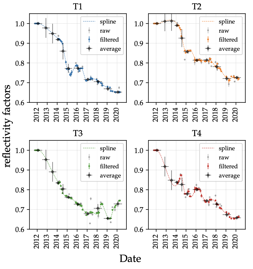
Figure 3: Time-dependent changes of the reflectivity factors obtained from WDR measurements. Black points show the average reflectivity factors for each instrument epoch. Blue, orange, green, and red points show the individual reflectivity factor measurements for each telescope. Curves of the same colors represent a spline interpolation, which removes outliers. The first point (early 2012) is extracted from the simulations and it serves as the reference for the calculation of the reflectivity factors, therefore adopting a value of 1 as reflectivity factor.We note that a value of the reflectivity factor slightly greater than 1 just means that the reflectivity at that time was slightly higher than at the time where simulations were produced.
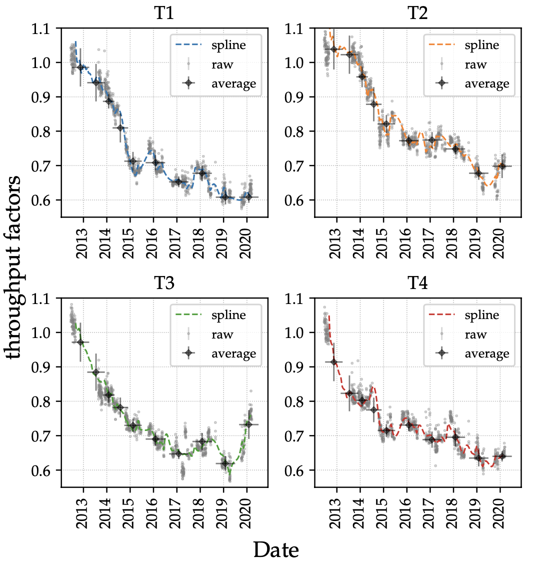
Figure 4: Time-dependent change of the throughput factors calculated from photo-statistic gain factors and WDR reflectivity factors. Error bars show only statistical uncertainties.
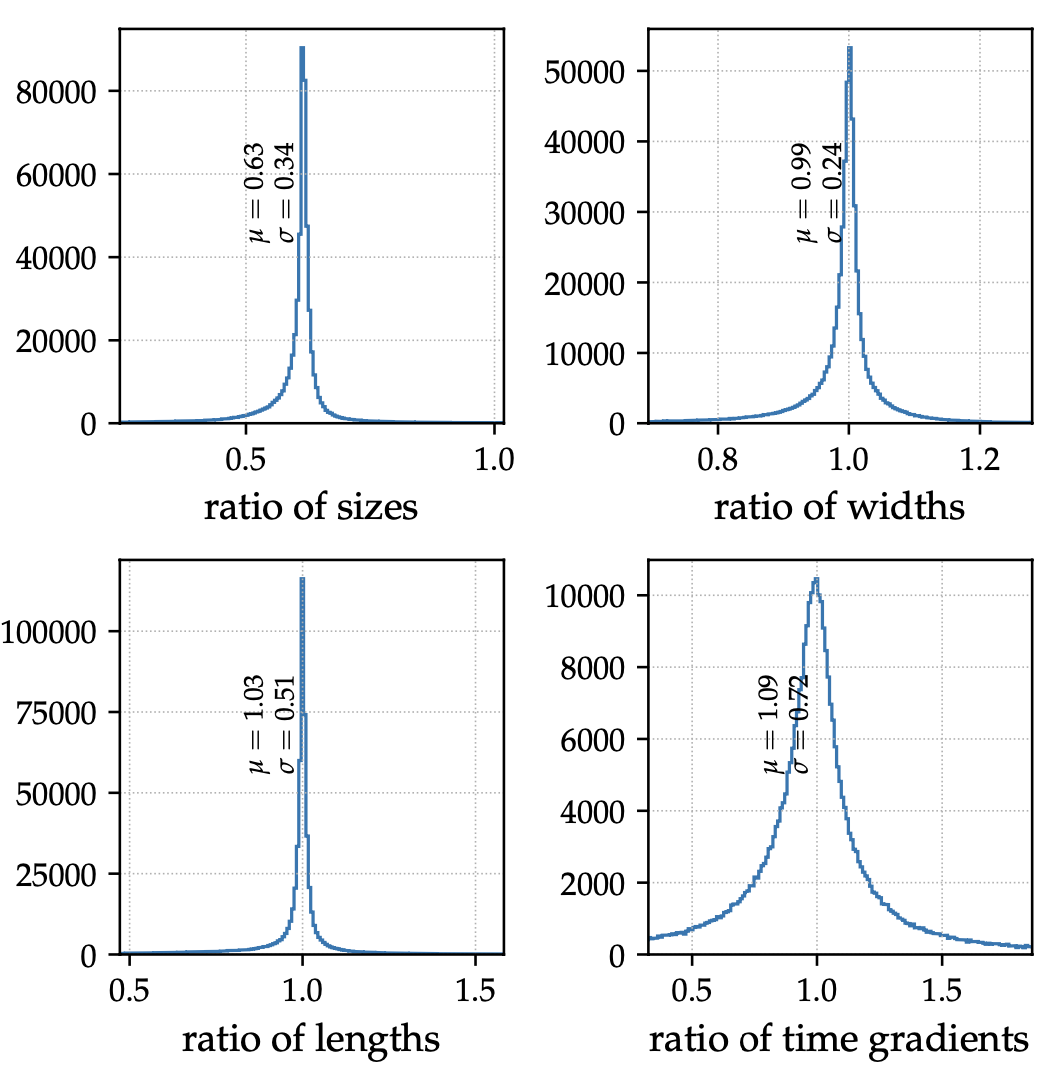
Figure 5: Ratio between image parameters derived from MC simulations for the season 2019-2020 vs season 2012-2013a (Telescope T1 only, winter simulations, noise level of 100 MHz, and no size cuts). The vertical axis of each panel shows the number of events within a given ratio bin.
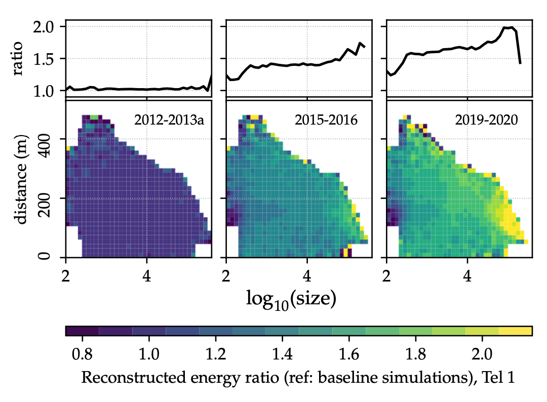
Figure 6: Relative changes in energy reconstruction induced by the evolution of the throughput of the instrument. The ratio of throughput calibrated energies with respect to the uncorrected energies is presented in two formats: As 2D lookup tables, with the ratio as function of impact distance and size of the simulated events (bottom panels); curves with the distance-averaged lookup-tables, showing the ratio as a function only of size (top panels).
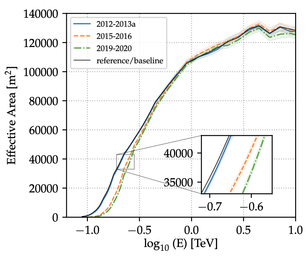
Figure 7: Evolution of the e�ffective area for diff�erent instrument epochs, for a zenith angle of observation of 20�, noise level of 100 MHz, moderate cuts and a minimum of two images per event.
Figure 8: Energy threshold of the analysis estimated from simulated events and using moderate cuts, zenith angle of 20�, and noise level of 100 MHz. It is defined as the energy for which the e�ffective area becomes 10% of the maximum e�ffective area.
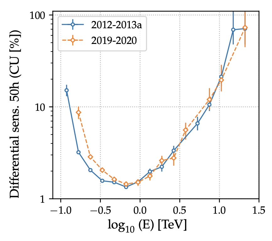
Figure 9: Diff�erential sensitivity with 50 h of VERITAS observations calculated using diff�erent low zenith angle Crab Nebula data, with winter atmospheric profile conditions. The same cuts as in Figure 7 are used. The sensitivity is defined in terms of the flux of the Crab Nebula (in Crab units, CU) assuming it is a reference astrophysical object at VHE energies.
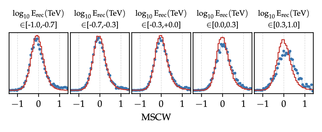
Figure 10: Average distributions of MSCW values, in di�fferent energy bins, for the data (blue points) and simulation (red curve) in the entire post-upgrade period. They were both generated after throughput calibration. Data events were obtained from a sample of Crab Nebula observations. Due to the small total number of events, the last two energy bins are combined into a single bin with energies log10 Erec(TeV) ∈ [0.3; 1.0].
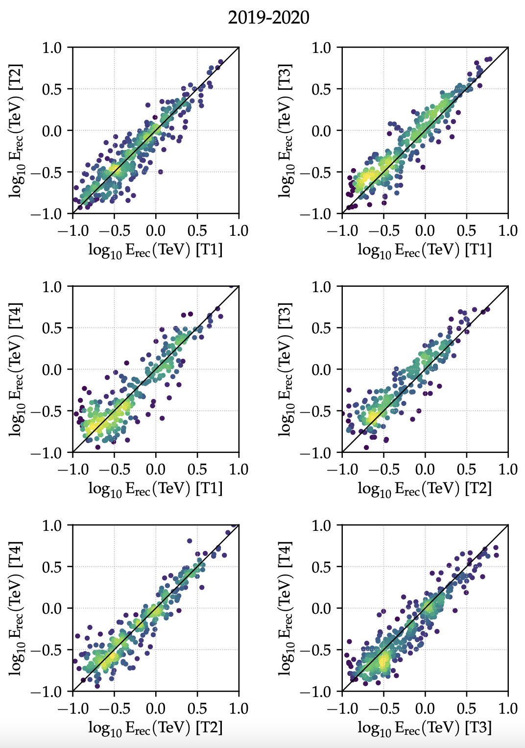
Figure 11: Inter-telescope calibration: reconstructed energies for γ-ray like events from Crab Nebula observations, with a similar (difference less than 20%) distance from each telescope to the reconstructed shower core. The density of events in the parameter space is color-coded, with yellow values representing more events and blue values representing fewer events. A 1:1 relationship for the event energies is plotted in black, corresponding to perfect inter-telescope calibration. For compactness, we only show the results for 2019-2020.
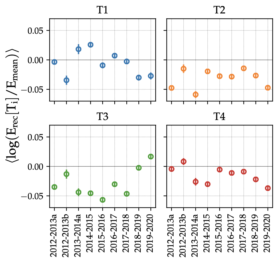
Figure 12: Mean of the log10 (Erec[Ti]=Emean) values for selected γ-ray-like events and its standard deviation, for each telescope and season, where Erec[Ti] is the reconstructed energy of telescope i and Emean the average reconstructed energy from the entire array, using the same weights for all telescopes. For a given epoch, the energies reconstructed by the di�fferent telescopes do not deviate on average more than ≈ 10% with respect to the mean energy reconstructed with the entire array.
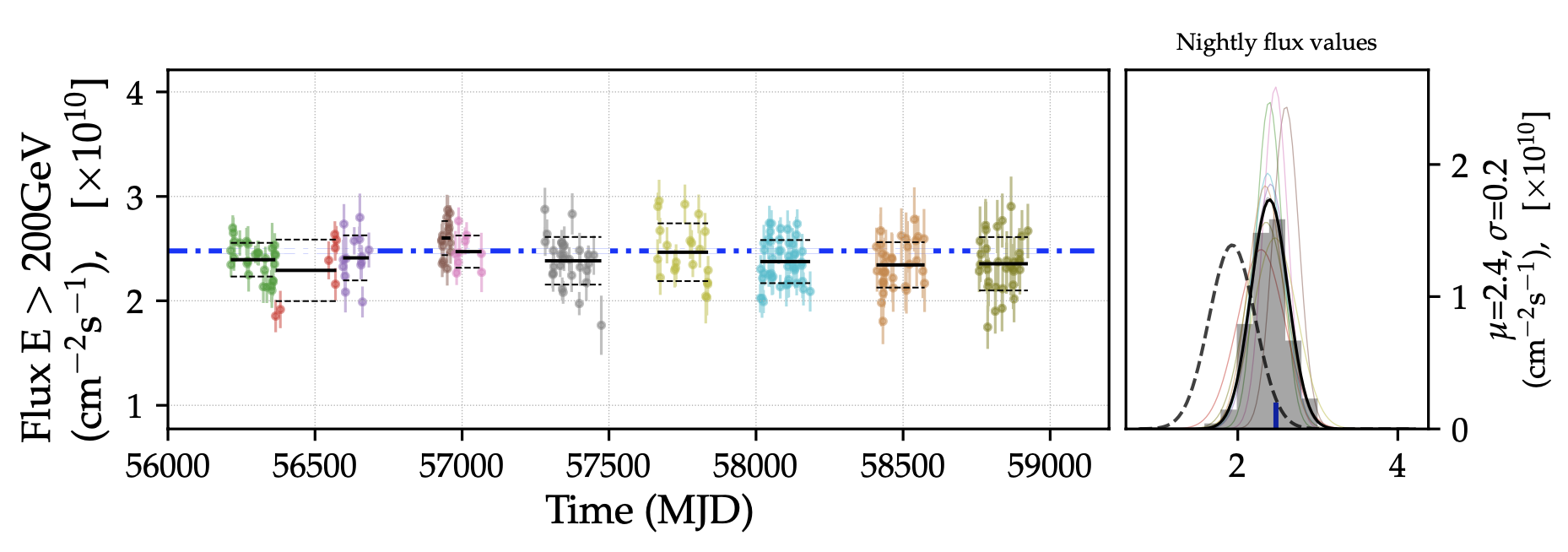
Figure 13: Reconstructed flux of the Crab Nebula above 200 GeV, using 1-day bins and IRFs that correctly match the instrument throughput for each period. Results are obtained applying moderate cuts to runs with mean elevation > 50o�. Left panel: Each color represents an IRF period. The blue dot-dashed curve represents the reference Crab Nebula spectrum of Meagher (2015) integrated above 200 GeV, horizontal solid black lines represent the season-average fluxes, while dashed horizontal curves show the standard deviation of the fluxes for each season. Right panel: Shown in gray is the distribution of fluxes for all seasons combined, with a fit to a Gaussian shape as a solid black line. The dashed black curve shows the equivalent result when throughput changes are not taken into account in the IRFs. The vertical blue dashed line shows the reference Crab Nebula flux from Meagher (2015).
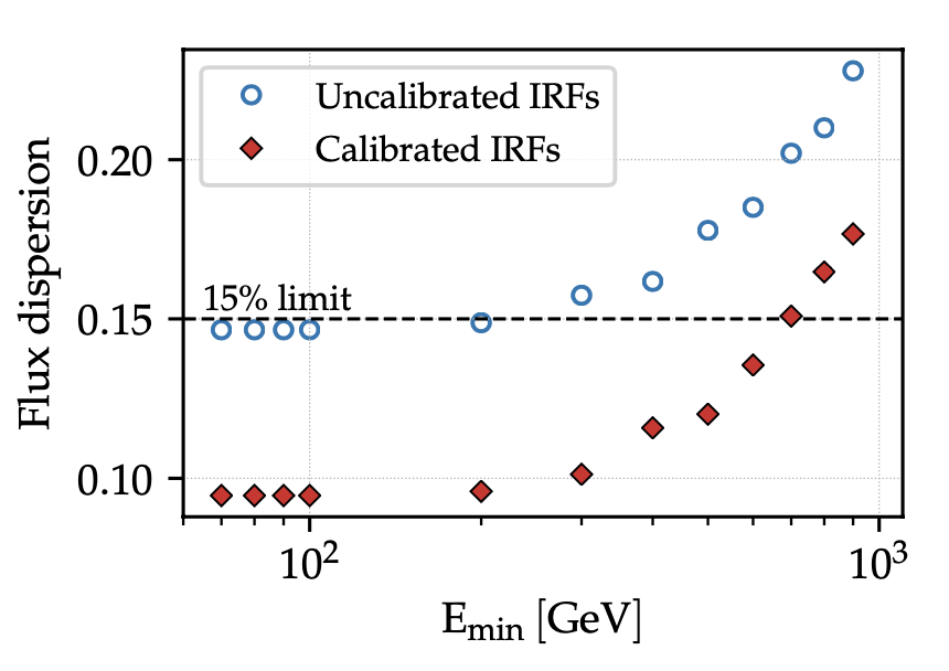
Figure 14: Flux dispersion (�σ/μ�) as a function of threshold energy for light curves similar to the one of Figure 13, using moderate cuts. Taking into account the throughput evolution brings down the statistical uncertainties from ≈�15% baseline to �≈10%.
Figure 15: Collection of spectral energy distributions obtained with moderate cuts for each IRF period. Purple open diamonds represent measurements of the Crab Nebula spectrum from the 3FHL (Ajello et al. 2017), the orange curve shows the Crab Nebula spectrum published by VERITAS in Meagher (2015), open blue points show the fluxes that would be obtained if throughput is not calibrated during the reconstruction of γ-ray showers and instead the MC model from 2012 is employed. Finally, red solid points show the spectral points that are obtained once the pulse signals are calibrated to generate correct IRFs for each period.